Form 3 Mathematics

Chapter 5: Functional Graphs

---

5.1. Introduction
5.2. Functional notation
5.2.1. Formation of the functional notation
5.2.2. Calculations in functional notation
5.3. Linear functions/graphs
5.3.1. Plotting a linear function/graph
5.3.2. Gradient of linear functions
5.3.3. Finding the gradient from the equation of a straight line
5.4. Cubic function/graph
5.4.1. Plotting the cubic function
5.4.2. Area under the curve
5.4.3. Gradient on a cubic function
5.4.4. Roots of a cubic function
5.4.5. Turning points of the cubic function
5.5. Summary
5.6. Further reading
5.7. Test 5

---

5.1. Introduction

Have you ever asked yourself why do we use graphs? Well you are not alone. The answer to the questions is that graphs give a pictorial view of information which may not be easily understood on its own. The pictorial presentation may even speak volumes of information which other methods of data presentation could not tell. In this chapter you will learn how to interpret the functional notation, plot functional graphs and calculate other aspects related to the functional graphs such as area under the graph, gradients and finding roots of intersecting lines. Figure 5.1 is an example of a graph.

Figure 5.1: Graph

Objectives

After going through this chapter, you should be able to

• use and interpret the functional notation.
• construct a table of values from a given function.
• use given scale correctly to construct the functions.
• draw graphs (functions) of the form
  • \( y = mx + c \) (linear function).
  • \( y = x^3 \) (cubic function).
• estimate the area under the curve.
• draw tangents at given points.
• estimate the gradient of lines and curves at given points.
• solve equations graphically.
• use graphs to determine the maximum and minimum turning points.

Key terms

Gradient – This is the measure of the steepness of a line.
Intersection – This is the point where two lines or curves meet or join.
Line of symmetry – The line which divides a shape (a curve in our case) into two equal parts.
Maximum – This is the highest of greatest point reached.
Minimum – This is the least value of the smallest value reached.
Tangent – This is a straight line which passes through a point on a curve, it just touches a curve at a point.

Time

You should not spend more than 10 hours in this chapter.

Study skills

You should have a graph book or graph paper for practice. The key to mastery of mathematics is practice. You need to work out as many problems as possible about functional graphs to have a better understanding of the subject.

5.2. Functional notation

5.2.1. Formation of the functional notation

Suppose you are given the expression x + 3 and then you are told that the value of x is 2. If you replace x with 2, what will be the value of the expression? The value will be 5. x + 3 is a rule which connects a number to another number. x + 3 is the rule connecting 2 to 5. The rule is called a function. Therefore x + 3 is a function. The letter ‘f’ denotes the function. The result of applying a function to a number is denoted by f(x). The above example can be expressed as f(x) = x + 3. The equation y = 6x + 5 can be written in functional notation as f(x) = 6x + 5. The inclusion of f(x) is what we call the functional notation.

Example 1

Questions

• Convert the following equations to functional notation.
  1. y = 2x + 4
  2. \( y = 4x^2 − 5x \)
  3. \( y = \dfrac{3x + 2}{2x + 1} \)

Answers

1. In the equation y = 2x + 4 you simply replace ‘y’ with f(x), it becomes f(x) = 2x + 4.
2. In the equation \( y = 4x^2 − 5x \) you simply replace again ‘y’ with f(x), it becomes \( f(x) = 4x^2 − 5x \).
3. In the equation \( y = \dfrac{3x + 2}{2x + 1} \) you simply replace again ‘y’ with f(x), it becomes \( f(x) = \dfrac{3x + 2}{2x + 1} \).

Convert the following equations to function notation, in the space provided.

1. y = 7x – 4
2. \( 5x^2 + 4x = y \)
3. \( y = \dfrac{x^2 + 4x}{3} \)

Hint: If you have just replaced ‘y’ with f(x) you got it right.

5.2.2. Calculations in functional notation

Let us use our functions/rule to find out how we can connect numbers or to find out other numbers. Consider the following examples.

Example 2

Questions

• Given that f(x) = 2x + 9, find
  1. f(0)
  2. f(3)
  3. f(-1)
  4. \( f(\dfrac{1}{2}) \)

Answers

Hint: You simply replace the value of x with the given value.

1. Replace the x value with ‘0’ in the function f(x) = 2x + 9.
   f(0) = 2(0) + 9
   f(0) = 0 + 9
   f(0) = 9
2. Replace the x value with ‘3’ in the function f(x) = 2x + 9.
   f(3) = 2(3) + 9
   f(3) = 6 + 9
   f(3) = 15
3. Replace the x value with ‘−1’ in the function f(x) = 2x + 9.
   f(−1) = 2(−1) + 9
   f(−1) = −2 + 9
   f(−1) = 7
4. Replace the x value with ‘\( -\dfrac{1}{2} \)’ in the function f(x) = 2x + 9.
   \( f(-\dfrac{1}{2}) = 2(-\dfrac{1}{2}) + 9 \)
   \( f(-\dfrac{1}{2}) = -1 + 9 \)
   \( f(-\dfrac{1}{2}) = 8 \)

Now let us consider an example which requires us to find the value of x given the outcome of using the function.

Example 3

Questions

• Given that f(x) = 2x + 4, find x if f(x) = 10.

Answers

• You are required to find the value of x which will result in the rule obtaining a 10. The value of x which will result in the rule obtaining a 10 is 3. Here is how we obtain the 3.
  
  f(x) = 2x + 4 and f(x) = 10
  since f(x) = f(x) it also implies that 2x + 4 = 10
  solve for x in the equation 2x + 4 = 10
  2x + 4 = 10
  2x = 10 - 4
  2x = 6
  x = 3

Example 4

Questions

• Given that f(x) = kx + 8, find k if f(2) = 12.

Answers

• You are told that if you substitute x with 2 in the given function the result should be 12. Therefore you just have to substitute x with 2 and equate to 12.
  f(x) = kx + 8 and that f(2) = 12
  substitute x with 2 and equate to 12
  f(2) = k(2) + 8 = 12
  
  observe that k(2) will have to be written as 2k
  2k + 8 = 12
  
  solve for k
  2k + 8 = 12
  2k = 12 − 8
  2k = 4
  k = 2

You may attempt the following exercise.

Exercise 5.1: Functional notation

Questions

1. Given that f(x) = x + 3, find
   1. f(0)
   2. f(−2)
   3. \( f(\dfrac{1}{2}) \)
2. Given that \( f(x) = x^2 − 3x − 10 \), find
   1. f(0)
   2. f(−1)
   3. the value of x if f(x) = 0
3. If \( f(x) = \dfrac{3x + 2}{x - 1} \), find
   1. f(2)
   2. x if f(x) = 4
4. Given that f(x) = kx + 12, find the value of k if f(2) = 24.
5. If \( f(x) = \dfrac{r + 3x}{rx + 1} \), find r if f(-2) = 1.
6. Given that \( f(x) = k^2x^2 − 3kx − 11 \), find the two values of k if f(1) = −1.

Answers

1. 1. 3
   2. 1
   3. 3.5
2. 1. -10
   2. -6
   3. x = 5 or x = -2
3. x = 8
4. x = 6
5. r = 2.5
6. k = 5 or k = -2

5.3. Linear functions/graphs

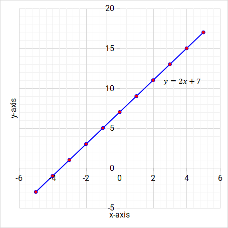
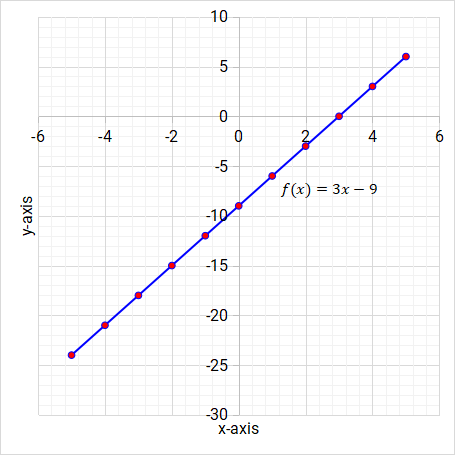
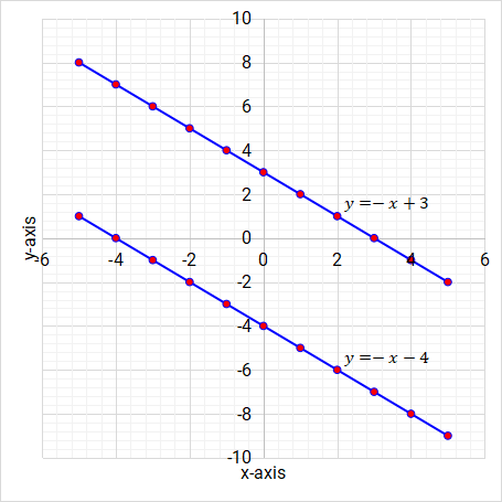
What are linear functions? Linear functions are straight line graphs. The highest power of the variable is 1. Here are a few examples of linear functions on Figure 5.2, Figure 5.3 and Figure 5.4.

Figure 5.2: Linear function/graph

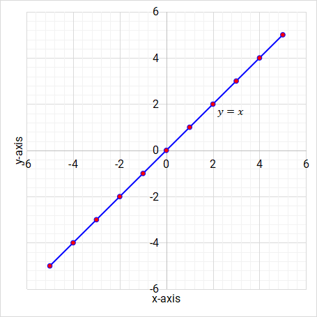
Figure 5.3: Linear function/graph

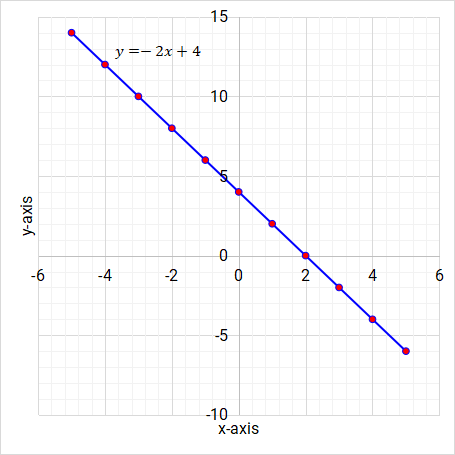
Figure 5.4: Linear function/graph

The highest power of the variable (x) in these linear functions examples is 1. Write any three examples of linear functions in the space provided.

5.3.1. Plotting a linear function/graph

Do you know how to plot a linear graph? If you don’t know, after going through the following example you will be well acquainted on how to plot or draw a straight line.

Note: In order to plot a graph of this nature, you should first draw up a table of values.

Example 5

Questions

• Plot the graph of y = 3x + 6. Use a scale of 2cm to represent 1 unit on the x−axis and 2 cm to represent 2 units on the y−axis.

Note: From the equation y = 3x + 6, the value of x is used to calculate the value of y. This means that x is the independent variable and y is the dependent variable.

Answers

• Step 1: Draw up a table of values.
  
  

  x
  y

  
  Step 2: Choose the values of x you would want to use.
  
  

  x	-1	0	1
  y

  
  Step 3: Calculate the values of y, and fill the table with values of x and y.
  We find the value of y by substituting the value of x in the given linear equation y = 3x + 6. We use the values of x chosen in step 2.
  
  When x = -1,
  y = 3x + 6
  y = 3(−1) + 6
  y = −3 + 6
  y = 3
  
  When x = 0,
  y = 3x + 6
  y = 3(0) + 6
  y = 0 + 6
  y = 6
  
  When x = 1,
  y = 3x + 6
  y = 3(1) + 6
  y = 3 + 6
  y = 9
  
  

  x	-1	0	1
  y	3	6	9

  
  Step 4: Using the proposed scale, mark the coordinates from the table of values onto the Cartesian plane.
  
  

  Figure 5.5: Linear function/graph

  

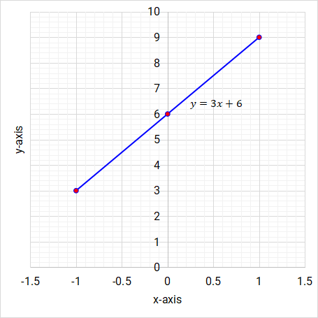
  Step 5: Join the coordinates using a ruler to produce a straight line and label the line.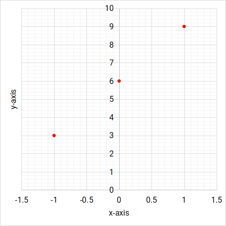
  
  

  Figure 5.6: Linear function/graph

  

Example 6

Questions

• Plot the graph of 5x + 2y = 10. Use a scale of 2cm to represent 1 unit for both the x−axis and y−axis.

Note: From the equation 5x + 2y = 10, make y the subject of formula so that you may use the values of x to calculate the values of y. The equation becomes \( y = \dfrac{10 - 5x}{2} \). This means that x is the independent variable and y is the dependent variable.

Answers

• Step 1: Draw up a table of values.
  
  

  x
  y

  
  Step 2: Choose the values of x you would want to use.
  
  

  x	-1	0	1
  y

  
  Step 3: Calculate the values of y, and fill the table with values of x and y.
  We find the value of y by substituting the value of x in the given linear equation \( y = \dfrac{10 - 5x}{2} \). We use the values of x chosen in step 2.
  
  When x = -1,
  \( y = \dfrac{10 - 5x}{2} \)
  \( y = \dfrac{10 - 5(-1)}{2} \)
  \( y = \dfrac{10 + 5}{2} \)
  \( y = \dfrac{15}{2} \)
  \( y = 7\dfrac{1}{2} \)
  
  When x = 0,
  \( y = \dfrac{10 - 5x}{2} \)
  \( y = \dfrac{10 - 5(0)}{2} \)
  \( y = \dfrac{10 - 0}{2} \)
  \( y = \dfrac{10}{2} \)
  \( y = 5 \)
  
  When x = 1,
  \( y = \dfrac{10 - 5x}{2} \)
  \( y = \dfrac{10 - 5(1)}{2} \)
  \( y = \dfrac{10 - 5}{2} \)
  \( y = \dfrac{5}{2} \)
  \( y = 2\dfrac{1}{2} \)
  
  

  x	-1	0	1
  y	\( 7\dfrac{1}{2} \)	\( 5 \)	\( 2\dfrac{1}{2} \)

  
  Step 4: Using the proposed scale, mark the coordinates from the table of values onto the Cartesian plane.
  
  

  Figure 5.7: Linear function/graph

  

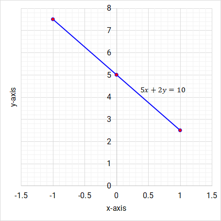
  Step 5: Join the coordinates using a ruler to produce a straight line and label the line.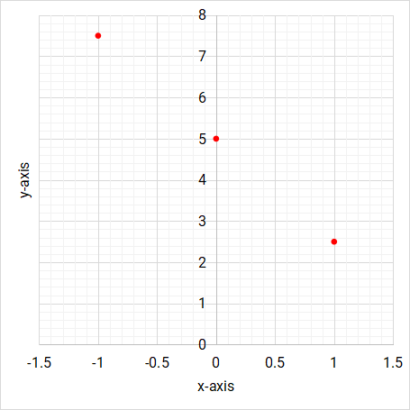
  
  

  Figure 5.8: Linear function/graph

  

You may attempt the following exercise.

Exercise 5.2: Line graphs

Questions

• Complete the table of values and plot the graphs for the following equations using an appropriate scale.
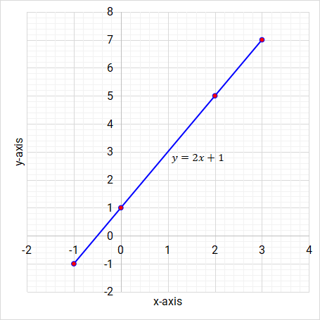
  1. y = 2x + 1
     
     

     x			2	3
     y	-1	1

     
     
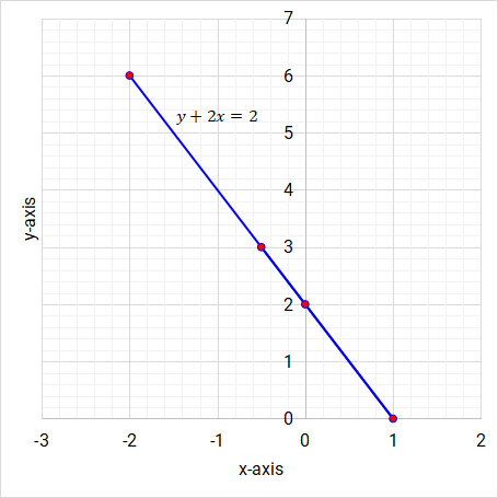
  2. y + 2x = 2
     
     

     x	-2	0
     y			0	3

     
     
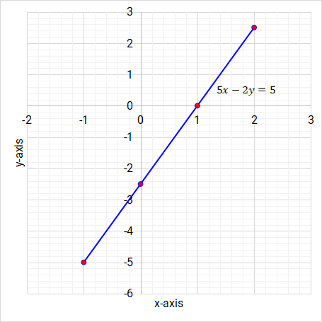
  3. 5x − 2y = 5
     
     

     x	-1	0	1	2
     y

     
     
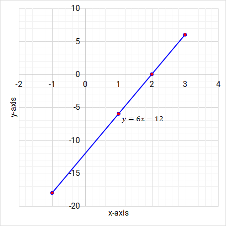
  4. y = 6x − 12
     
     

     x	-1			3
     y		-6	0

     
     

Answers

1. y = 2x + 1
   
   

   x	-1	0	2	3
   y	-1	1	5	7

   
   

   Graph y = 2x + 1

   

2. y + 2x = 2
   
   

   x	-2	0	1	-0.5
   y	6	2	0	3

   
   

   Graph y + 2x = 2

   

3. 5x − 2y = 5
   
   

   x	-1	0	1	2
   y	-5	-2.5	0	2.5

   
   

   Graph 5x - 2y = 5

   

4. y = 6x − 12
   
   

   x	-1	1	2	3
   y	-18	-6	0	6

   
   

   Graph y = 6x - 12

   

5.3.2. Gradient of linear functions

Gradient is defined as the rate of change in y compared to the rate of change in x. Gradient can either be positive or negative. If the rate of change in y moves in the same direction as the rate of change in x, then the gradient is positive. If the rate of change in y moves in the opposite direction as the rate of change in x, then the gradient is negative. The following graphs show lines which have positive gradient and those which have negative gradient.

Figure 5.13: Positive gradient

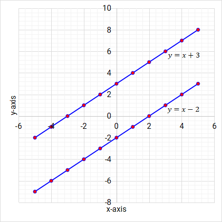
Figure 5.14: Negative gradient

We can obtain gradient of a line from

1. two given coordinates on the line, or
2. the equation of the straight line, or
3. two given coordinates.

The definition says gradient is the change of y compared to the change in x. The change in y is the difference between y values and we can denote that by saying \( y_1 - y_0 \). The change in x is also denoted by saying \( x_1 - x_0 \). This will then result in the formula for gradient written as

• \( Gradient = \dfrac{y_1 - y_0}{x_1 - x_0} \)

Using that formula, given two coordinates in the form (x, y), the gradient of a straight line can be calculated.

Example 7

Questions

• Find the gradient of the line passing through the following coordinates.
  1. (0, 4) and (–2, 0)
  2. (–2, –4) and (2, 8)
  3. (–1, 3) and (1, –1)

Answers

1. (0, 4) and (–2, 0)
   Identify your \( y_1 \), \( y_0 \) and \( x_1 \), \( x_0 \).
   \( y_1 = 0 \), \( y_0 = 4 \), \( x_1 = -2 \), \( x_0 = 0 \)
   
   \( Gradient = \dfrac{y_1 - y_0}{x_1 - x_0} \)
   \( Gradient = \dfrac{0 - 4}{-2 - 0} \)
   \( Gradient = \dfrac{-4}{-2} \)
   \( Gradient = 2 \)
   
2. (–2, –4) and (2, 8)
   Identify your \( y_1 \), \( y_0 \) and \( x_1 \), \( x_0 \).
   \( y_1 = 8 \), \( y_0 = -4 \), \( x_1 = 2 \), \( x_0 = -2 \)
   
   \( Gradient = \dfrac{y_1 - y_0}{x_1 - x_0} \)
   \( Gradient = \dfrac{8 - -4}{2 - -2} \)
   \( Gradient = \dfrac{12}{4} \)
   \( Gradient = 3 \)
   
3. (–1, 3) and (1, –1)
   Identify your \( y_1 \), \( y_0 \) and \( x_1 \), \( x_0 \).
   \( y_1 = -1 \), \( y_0 = 3 \), \( x_1 = 1 \), \( x_0 = -1 \)
   
   \( Gradient = \dfrac{y_1 - y_0}{x_1 - x_0} \)
   \( Gradient = \dfrac{-1 - 3}{1 - -1} \)
   \( Gradient = \dfrac{-4}{2} \)
   \( Gradient = -2 \)
   

5.3.3. Finding the gradient from the equation of a straight line

If given a straight line in the form y = mx + c, m represents the gradient of the line and c represents the y intercept. The y intercept is point at which the line touches or crosses the y−axis. If given a straight line in the form ax + by = c, to find the gradient, make y the subject of the formulae.

Example 8

Questions

• Find the gradient of the straight line represented by the following equations.
  1. y = -2x + 4
  2. 2y = 4x - 10
  3. 2x + 3y = 6

Answers

1. In the equation y = −2x + 4, y is already the subject of the formula. The gradient is the coefficient of x which is –2. Therefore the gradient is –2.
2. In the equation 2y = 4x - 10, we must make y the subject of the formula.
   2y = 4x − 10 (divide both by 2)
   \( \dfrac{2y}{2} = \dfrac{4x - 10}{2} \)
   \( y = \dfrac{4x - 10}{2} \)
   \( y = \dfrac{4x}{2} - \dfrac{10}{2} \)
   \( y = 2x - 5 \)
   The gradient is the coefficient of x which is 2. Therefore the gradient is 2.
3. In the equation 2x + 3y = 6, we must make y the subject of the formula.
   2x + 3y = 6 (rearrange)
   3y = 6 - 2x (divide both by 3)
   \( \dfrac{3y}{3} = \dfrac{6 - 2x}{3} \)
   \( y = \dfrac{6 - 2x}{3} \)
   \( y = \dfrac{6}{3} - \dfrac{2x}{3} \)
   \( y = 2 - \dfrac{2}{3}x \)
   The gradient is the coefficient of x which is \( -\dfrac{2}{3} \). Therefore the gradient is \( -\dfrac{2}{3} \).

You may attempt the following exercise.

Exercise 5.3: Gradient of a straight line

Questions

1. Find the gradient of the line passing through the following coordinates.
   1. (5, 4) and (0, 0)
   2. (6, –5) and (2, 3)
   3. (–3, 1) and (4, 3)
2. Find the gradient of the straight line represented by the following equations.
   1. -3y = 6x - 12
   2. 2y = 3x + 4
   3. 3x + 4y = 8
   4. 5x - 2y = -6

Answers

1. 1. \( \dfrac{4}{5} \)
   2. -2
   3. \( \dfrac{2}{7} \)
2. 1. -2
   2. 1.5
   3. -0.75
   4. 2.5

5.4. Cubic function/graph

In a cubic function, the highest power of the variable is 3, for examples \( y = x^3 \), \( y = 2x^3 + x^2 \) and \( y = 4x - x^3 \).

Figure 5.15: Cubic function/graph

The cubic function has two turning points.

5.4.1. Plotting the cubic function

These are the steps followed when plotting a cubic function.

• Draw up a table of values.
• Plot coordinates.
• Join the coordinates with a smooth curve.

Example 9

Questions

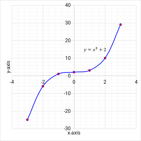
1. Complete the following table of values for \( y = x^3 + 2 \).
   
   

   x	-3	-2	-1	0	1	2	3
   y			1	2	3

   
   
2. Plot the graph of \( y = x^3 + 2 \). Use a scale of 2cm to represent 1 unit on the x-axis and 2cm to represent 5 units on the y-axis.

Answers

1. Find the missing values. Remember we substitute the x value to get the y value.
   When x = −3,
   \( y = x^3 + 2 \)
   \( y = -3^3 + 2 \)
   \( y = -27 + 2 \)
   \( y = -25 \)
   
   When x = −2,
   \( y = x^3 + 2 \)
   \( y = -2^3 + 2 \)
   \( y = -8 + 2 \)
   \( y = -6 \)
   
   When x = 2,
   \( y = x^3 + 2 \)
   \( y = 2^3 + 2 \)
   \( y = 8 + 2 \)
   \( y = 10 \)
   
   When x = 3,
   \( y = x^3 + 2 \)
   \( y = 3^3 + 2 \)
   \( y = 27 + 2 \)
   \( y = 29 \)
   
   

   x	-3	-2	-1	0	1	2	3
   y	-25	-6	1	2	3	10	29

   
   Using the proposed scale, mark the coordinates from the table of values onto the Cartesian plane.
   
   

   Figure 5.16: Cubic function/graph

   

   Join the coordinates with smooth lines and label the line.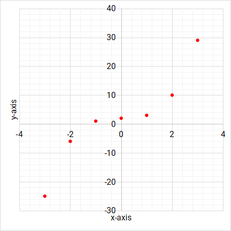
   
   

   Figure 5.17: Cubic function/graph

   

5.4.2. Area under the curve

The area enclosed by the curve and other given lines is calculated using either the trapezium or counting squares method.

Example 10

Questions

• The following is the graph of \( y = x^3 + 4x + 2 \).
  
  

  Figure 5.18: Cubic function/graph

  

  On the graph, calculate the area bounded by the curve, x-axis, x = 1 and x = 3.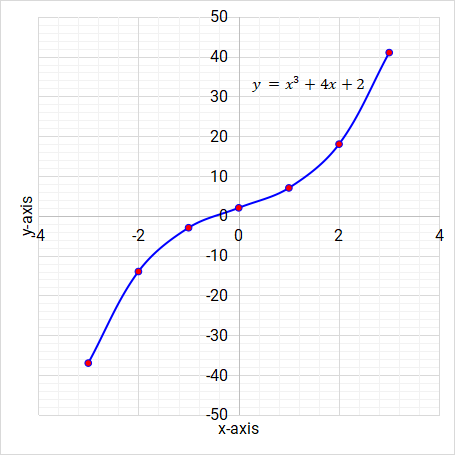

Answers

• Use the graph to mark the area bounded by the curve, x-axis, x = 1 and x = 3.
  
  

  Figure 5.19: Cubic function/graph

  

  On the graph, calculate the area bounded by the curve, x-axis, x = 1 and x = 3. Counting squares method: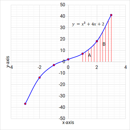
  \( 0.1 \times 1 \times 450 = 45 units^2 \)
  
  Trapezium method:
  \( Area \ A = \dfrac{1}{2}(7 + 22) = 14.5 \ units^2 \)
  \( Area \ B = \dfrac{1}{2}(22 + 41) = 31.5 \ units^2 \)
  \( Total \ Area = Area \ A + Area \ B \)
  \( Total \ Area = 14.5 \ units^2 + 31.5 \ units^2 \)
  \( Total \ Area = 46 \ units^2 \)

5.4.3. Gradient on a cubic function

These are the steps followed when calculating the gradient on a cubic function.

• Draw a tangent on the point in question.
• Calculate gradient using either one of the two methods.
  • Use two (x, y) coordinates on the tangent line.
  • Draw a right-angled triangle.

Example 11

Questions

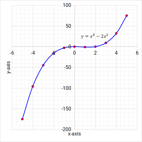
• The following is the graph of \( y = x^3 - 2x^2 \).
  
  

  Figure 5.20: Cubic function/graph

  

  On the graph, calculate the gradient at the point x = -1.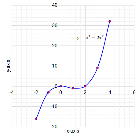

Answers

• Use the graph to draw a tangent passing through the point x = -1.
  
  

  Figure 5.21: Cubic function/graph

  

  On the graph, the gradient can then be calculated through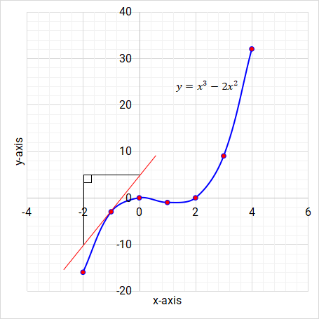
  Coordinates on the tangent line:
  The coordinates are (0, 5) and (–2, –10).
  \( y_1 = -10 \), \( y_0 = 5 \), \( x_1 = -2 \), \( x_0 = 0 \)
  
  \( Gradient = \dfrac{y_1 - y_0}{x_1 - x_0} \)
  \( Gradient = \dfrac{-10 - 5}{-2 - 0} \)
  \( Gradient = \dfrac{-15}{-2} \)
  \( Gradient = 7.5 \)
  
  Right-angled triangle:
  \( Gradient = \dfrac{y-axis length}{x-axis length} \)
  \( Gradient = \dfrac{15}{2} \)
  \( Gradient = 7.5 \)
  

5.4.4. Roots of a cubic function

In the cubic function, usually when a straight line intersects a cubic function we get three roots. Let us look at how we can find the roots.

Example 12

Questions

• The following is the graph of \( y = x^3 + 4x + 2 \).
  
  

  Figure 5.22: Cubic function/graph

  

  Using the graph, find the roots of the equation \( 0 = x^3 + 4x + 2 \).

Answers

• Subtract the equation \( 0 = x^3 + 4x + 2 \) from the original function \( y = x^3 + 4x + 2 \).
  
  \( \begin{array}{r}\phantom{0}y = x^3 + 4x + 2 \\ -0 = x^3 + 4x + 2 \\ \hline \phantom{0}y - 0 = x^3 - x^3 + 4x - 4x + 2 - 2 = 0 \phantom{0} \end{array} \)
  
  This gives y = 0.
  Draw the line y = 0 on the same axis.
  
  

  Figure 5.23: Cubic function/graph

  

  The line will intersect the curve at a point where the root is -0.6.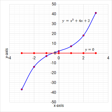

5.4.5. Turning points of the cubic function

A cubic function has two turning points, that is, a maximum and a minimum (and a saddle which is beyond the scope of this level).

Example 13

Questions

• The following is the graph of \( y = 3x - x^3 \).
  
  

  Figure 5.24: Cubic function/graph

  

  Using the graph, write down the coordinates of the turning points.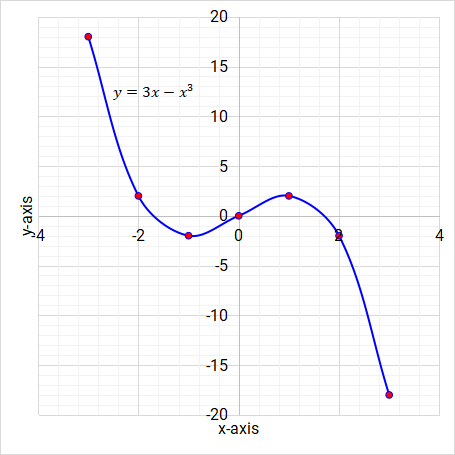

Answers

• There are two turning points on the graph.
  • The maximum turning point coordinates are (1, 2).
  • The minimum turning point coordinates are (–1, –2).

You may attempt the following exercise.

Exercise 5.4: Cubic functions

Questions

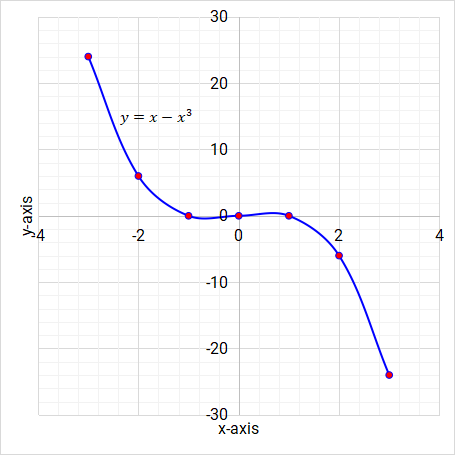
1. The following is an incomplete table of values for \( y = x − x^3 \).
   
   

   x	-3	-2	-1.5	0	1.5	2	3
   y	a	6	1.9	0	b	-6	-24

   
   
   1. Find the value of a and b.
   2. Using a scale of 2cm to represent 1 unit on the x-axis and 2 cm to represent 5 units on the y-axis, draw the graph of \( y = x − x^3 \).
   3. Use your graph to
      1. find the gradient of the curve at the point x = ?
      2. write down the coordinates of the maximum turning point.
      3. find the roots of the equation \( x − x^3 = 0 \).
      4. solve the equation \( 2 − 2x = x − x^3 \).
   4. Estimate, using your graph the area enclosed by the curve, the x − axis, the lines x = 1 and x = 3.
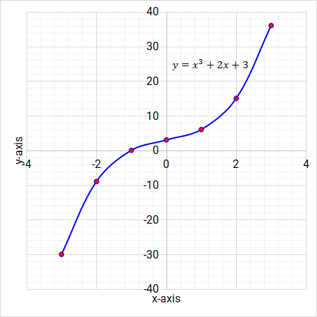
2. The following is an incomplete table of values for \( y = x^3 + 2x + 3 \).
   
   

   x	-4	-3	-2	-1	0	1	2	3	4
   y		m					n

   
   
   1. Find the values of m and n.
   2. Using a scale of 2cm to represent 1 unit on the x-axis and 2cm to represent 5 units on the y–axis, draw the graph of \( y = x^3 + 2x + 3 \).
   3. Using your graph,
      1. find the gradient of the curve at x = 2.
      2. find the roots of the equation \( y = x^3 + 2x + 3 \).
      3. state the values of y at the turning points.
   4. Calculate an estimate of the area enclosed by the curve, the x-axis, the lines x = −2 and x = −3.
   5. Show on the graph the region for which we will calculate the area.

Answers

1. 1. a = 24, b = -1.9

   2. Figure 5.25: Cubic function/graph

      

   3. 1. -3.75
      2. There is no maximum or minimum turning points. It is a saddle, which is beyond the scope of this level.
      3. x = 0
      4. -1.55
   4. \( 15 \ units^2 \)
2. 1. m = -28, n = 15

   2. Figure 5.26: Cubic function/graph

      

   3. 1. 12.5
      2. x = −1
      3. There is no turning point
   4. \( 18.5 \ units^2 \)

5.5. Summary

In this chapter we learnt about how to interpret the functional notation, construct a table of values from a given function, use a given scale correctly to construct graphs (functions) of the form y = mx + c for a linear function and \( y = x^3 \) for a cubic function. We also learnt how to calculate the gradient of a linear function, estimate the area under the curve, draw tangents at given points, estimate the gradient of curves at given points, solve equations graphically and use graphs to determine the maximum and minimum turning points.

5.6. Further reading

1. Macrae, M. F., Madungwe, L. and Mutangadura, A. (2017). New General Mathematics Book 3. Pearson Capetown.
2. Macrae, M. F., Madungwe, L. and Mutangadura, A. (2017). New General Mathematics Book 4. Pearson Capetown.
3. Meyers, C., Graham, B., Dawe, L. (2004). Mathscape Working Mathematically. 9th Edition. MacMillan.
4. Pimentel, R. and Wall, T. (2011). International Mathematics. Hodder UK.
5. Rayner, D. (2005). Extended Mathematics. Oxford New York.

5.7. Test 5